The Economist’s Presidential election model might not get quite as much publicity as the FiveThirtyEight model or Nate Silver’s latest vehicle, but it’s been going since 2020, and has perhaps the most solid statistical pedigree of all.
Its family tree is detailed and somewhat knotted, but the 2024 version can have few equals in terms of intellectual heft. It is based on the previous versions (written by G. Elliot Morris, now at FiveThirtyEight), but now fully credited to Andrew Gelman - the eminence grise of Bayesian statistics, with Ben Goodrich, his Columbia colleague, lending expertise the political science side.
How does it work?
The Economist’s explanation of the model, for my money, one of the more appallingly structured article on the workings of a model you’ll ever see. The article proceeds chronologically through the steps, talking about historical data and various regression techniques, but this means we are more than 75% through the article by the time it mentions that what we are building is a Bayesian model, and everything we have read so far is about constructing a prior.
For comparison, this would be like an article about a building project spending 75% of the time talking about pouring the foundations, and only at that point mentioning in passing that we’re building La Sagrada Familia.
The foundations are important - no argument there - but what you’re doing makes very little sense without the context of the whole structure.
Rockets and unknowns
Let’s try to lay out a sketch of this structure. As made clear in the last couple of paragraphs of the Economist article, the model is fully Bayesian. It brings together a “prior” - which is derived from historical voting patterns, state-level polling (adjusted a bit), and updates it with national-level polling (adjusted a bit) as well as state-level polling (adjusted a bit), with all this updating dealt with by something called a dynamic linear model1 to try to sort out what the most likely true state of the race is, and how it could evolve between now and polling day.
The basic method for how you “throw them” together is the core of the model, and it has an interesting history. It was originally studied in the context of control theory, and in particular controlling rockets in the space race.
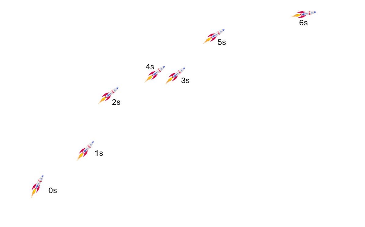
Let’s imagine we have some radar reads on a rocket, every second or so. These reads are not completely accurate, they are usually right to within some radius of a few kilometers, which we either know, or can guess.
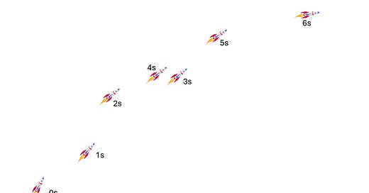
Let’s say - raw - the radar fixes on the position look like this:
We also know some stuff about the rocket’s engine, when it’s firing and when it’s not. We also know basic Newtonian physics which tells us - for example - that it’s pretty unlikely that the rocket actually did manage to go backwards between between 3 and 4 seconds.
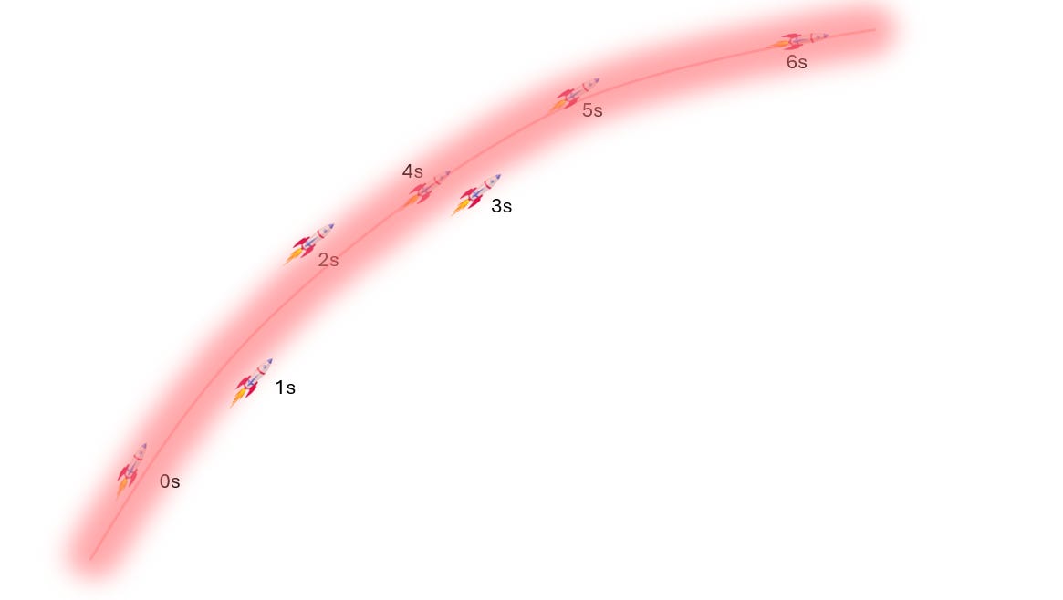
Nonetheless, these are the observations we have, with some error rates, these are the dynamics we know, and we are trying to derive our best guess of the “hidden state” of the rocket - which is its real, unobserved location over time.
Rudolf Kalman was the first to come up with a method that allows you to throw all these measurements ,their uncertainty and known dynamics into a series of equations, and have the mathematics spit out the most likely path of the rocket, plus error bars on this path.
What’s more, it allowed you to update these estimates with each new read that came in - exactly what you need to track a rocket with error-prone radar readings. As such, its first application was in the Apollo programme in the 1960s, and then - less inspiringly - in cruise missiles and submarine tracking. Since Kalman, and his “Kalman filter” - which is well-known to control systems engineers,2 further approaches have been put forward, including various the fully Bayesian methodologies used by The Economist and its sister models.
Over to elections
You might have already noticed that this basic framework is exactly what we need to try to derive the true state of public opinion from a bunch of noisy polling data. Our “noisy, error-prone” observations are the national and state polling, our “dynamics” are how individual states tend to track the national picture and how fast public opinion tends to drift over time. And our “hidden state”, or the “position of the rocket” is the share of the voting public over time who will vote for Harris or Trump, both nationally and in each state.
The dynamics of an entire election are pretty complex - you need to derive how state polling tracks the national level (e.g., Michigan polling is expected to be much closer to the national level than Kansas) and the historical track record will only get you a certain way. Demographics, race and income level all have an effect. Then you are dealing with errors and “house effects” from individual pollsters, as well as their unknown biases and sampling errors. But - in principle - you can code up all this dynamics, all these inputs, throw them all into a Dynamic Linear Model, and ask the maths to sort it all out and derive the “hidden state”. That is, to derive a value for true underlying public opinion over time, as well as the error bars.
And this is exactly what they have done.
What’s more, this line - just like the track of the rocket - can be updated regularly with new “observations” i.e., new polling. And this updates its beliefs about the past as well as the future. For example, if you poll Texas one day and it has Trump +5, but you poll it the next week and it has Trump +10, that will increase the model’s belief that the first +5 reading was actually under-calling his true lead. So this “ripples” back through the history of the model, as well as changing its read about the future.


